4: Circular Whole Genome Comparison

Author

Richard Goodman

Published

April 24, 2025

Introduction

This tutorial will take two genome sequences and run a blastn comparison then visualise the comparison as a circlize output

This workflow involves using BLAST for sequence alignment, parsing the results, and visualizing the differences using circlize in R.

For a more in-depth tutorial on circular whole genome comparison see my circular genome comparisons github repo.

Part 1 - Genome download and comparison in bash

1.1: Download reads and run assemblies

See the code on how to download reads and run assemblies

1.2: Download reads and run assemblies

You should now have the following files which we cna use for the tutorial

FSBL1386_hybracter.fasta
FSFC1386_hybracter.fasta

1.3: Rename all contig headers i.e. everything after the “>”

Pattern breakdown:

^(>[^ ]+) → Captures the initial sequence identifier (e.g., >NZ_CP102708.1).
.* (chromosome|plasmid [^,]+) → Captures the desired terms:
chromosome (single word).
plasmid [^,]+ (the full plasmid name before a comma or end of the line).
\2 → Replaces the header with the extracted part.

Second sed step: * s/ //g → Replaces spaces with underscores. * s/^>/>9A-3-9/ → Adds the prefix to all headers.

Note: this pattern is specific to these fasta files, use a different syntax for different headers


# Check fasta headings
grep "^>" *.fasta

# For single files
sed -E 's/^(>[^ ]+) .* (chromosome|plasmid [^,]+).*/>\2/' FSBL1386.fasta | sed -E 's/ /_/g; s/^>/>FSBL1386_/' > FSBL1386.fasta
sed -E 's/^(>[^ ]+) .* (chromosome|plasmid [^,]+).*/>\2/' FSFC1386.fasta | sed -E 's/ /_/g; s/^>/>FSFC1386_/' > FSFC1386.fasta

# For multiple files
for file in *.fasta; do
    base=$(basename "$file" .fasta)
    sed -E 's/^(>[^ ]+) .* (chromosome|plasmid [^,]+).*/>\2/' "$file" | \
    sed -E "s/ /_/g; s/^>/>${base}_/" > "${base}.fasta"
done

# Check fasta headings again
grep "^>" *.fasta

1.4: Install seqkit

Make sure you have seqkit installed. You can download it from Wei Shen’s Github page.

1.5: Use seqkit to get contig length


seqkit fx2tab -n -l FSBL1386_hybracter.fasta > FSBL1386_lengths.tsv

seqkit fx2tab -n -l FSFC1386_hybracter.fasta > FSFC1386_lengths.tsv

1.6: Install BLAST

Make sure you have BLAST installed. You can download it from the NCBI BLAST website.

1.7: Use BLAST to align the sequences

Use BLAST to align the sequences in the FASTA files.

# Define your reference and query genomes
REF=FSFC1386_hybracter.fasta
Q= FSBL1386_hybracter.fasta

# Check your reference and query genomes
$REF
$Q

# Create BLAST databases for both genomes
makeblastdb -in ${REF} -dbtype nucl -out ${REF}_db

makeblastdb -in ${Q} -dbtype nucl -out ${Q}_db

# Perform QAST to compare genome1 to genome2
blastn -query ${REF} -db ${Q}_db -out ${REF}_vs_${Q}.blastn -outfmt 6

# Perform BLAST to compare genome2 to genome1
blastn -query ${Q} -db ${REF}_db -out ${Q}_vs_${REF}.blastn -outfmt 6

Part 2 - Visulisation with circulize in R

2.1: Parse the BLAST results to get the alignments

Parse BLAST Results

Parse the BLAST results to get the alignments.

# Load necessary libraries
library(Biostrings)
library(dplyr)
library(circlize)
library(colorspace)

parse_blast <- function(blast_file) {
  blast_data <- read.table(blast_file, header = FALSE, stringsAsFactors = FALSE)
  colnames(blast_data) <- c("qseqid", "sseqid", "pident", "length", "mismatch", 
                            "gapopen", "qstart", "qend", "sstart", "send", 
                            "evalue", "bitscore")
  return(blast_data)
}

blast_data <- parse_blast("../BLAST_data/FSBL1386_vs_FSFC1386.blastn")

blood = "FSBL1386"
faecal = "FSFC1386"

head(blast_data)

                    qseqid                   sseqid  pident  length mismatch
1 FSBL1386_chromosome00001 FSFC1386_chromosome00001 100.000 3341929        0
2 FSBL1386_chromosome00001 FSFC1386_chromosome00001 100.000 1998734        0
3 FSBL1386_chromosome00001 FSFC1386_chromosome00001  98.864    5548       43
4 FSBL1386_chromosome00001 FSFC1386_chromosome00001  98.864    5548       43
5 FSBL1386_chromosome00001 FSFC1386_chromosome00001  99.661    5316       16
6 FSBL1386_chromosome00001 FSFC1386_chromosome00001  99.661    5316       16
  gapopen  qstart    qend  sstart    send evalue bitscore
1       0 1999234 5341162       1 3341929      0  6171000
2       0       1 1998734 3341930 5340663      0  3691000
3      18 5152335 5157877 2247379 2252911      0     9878
4      18 4246612 4252144 3153102 3158644      0     9878
5       2 5015767 5021081 2629611 2634925      0     9716
6       2 4628844 4634158 3016534 3021848      0     9716

2.2: Get genome lengths from seqkit table

# Load necessary libraries
library(dplyr)

# Read contig lengths from the seqkit output
contig_lengths_ref <- read.table("../BLAST_data/FSBL1386_lengths.tsv", header = FALSE, sep = "\t", stringsAsFactors = FALSE)
contig_lengths_q <- read.table("../BLAST_data/FSFC1386_lengths.tsv", header = FALSE, sep = "\t", stringsAsFactors = FALSE)

contig_lengths = rbind(contig_lengths_ref, contig_lengths_q)

colnames(contig_lengths) <- c("chr", "length")

# Inspect the data
head(contig_lengths)

                                                                                                               chr
1                                                               FSBL1386_chromosome00001 len=5341162 circular=true
2  FSBL1386_plasmid00001 length=143420 plasmid_copy_number_short=0.9x plasmid_copy_number_long=0.49x circular=true
3                                                                             FSFC1386_chromosome00001 len=5340663
4 FSFC1386_plasmid00001 length=143423 plasmid_copy_number_short=0.56x plasmid_copy_number_long=3.34x circular=true
5   FSFC1386_plasmid00002 length=6415 plasmid_copy_number_short=11.89x plasmid_copy_number_long=0.0x circular=true
   length
1 5341162
2  143420
3 5340663
4  143423
5    6415

# Update genome length table with actual contig sizes
genome_lengths <- contig_lengths %>%
  dplyr::mutate(start = 0, end = length) %>%
  dplyr::select(chr, start, end)

# Add dummy numeric column as before
genome_lengths$value <- 1

2.3: Rename genome lengths

# rename to make contigs simpler
genome_lengths$chr = gsub("chromosome0000", "chr", genome_lengths$chr)
genome_lengths$chr <- gsub("plasmid0000", "p", genome_lengths$chr)
genome_lengths$chr <- gsub("FS", "", genome_lengths$chr)
genome_lengths$chr <- gsub("_", " ", genome_lengths$chr)
genome_lengths$chr <- gsub("1386", "", genome_lengths$chr)

# Remove anything after "len=" or "length="
genome_lengths$chr <- gsub("(len(gth)?).*", "", genome_lengths$chr)
genome_lengths$chr <- gsub("(?<=\\d)\\s", "", genome_lengths$chr, perl = TRUE)

# Check final genome lengths table
print(genome_lengths$chr)

[1] "BL chr1" "BL p1"   "FC chr1" "FC p1"   "FC p2"

2.4: Rename BLAST data

# rename to make contigs simpler
blast_data$qseqid = gsub("chromosome0000", "chr", blast_data$qseqid)
blast_data$qseqid <- gsub("plasmid0000", "p", blast_data$qseqid)
blast_data$qseqid <- gsub("FS", "", blast_data$qseqid)
blast_data$qseqid <- gsub("_", " ", blast_data$qseqid)
blast_data$qseqid <- gsub("1386", "", blast_data$qseqid)


# rename to make contigs simpler
blast_data$sseqid = gsub("chromosome0000", "chr", blast_data$sseqid)
blast_data$sseqid <- gsub("plasmid0000", "p", blast_data$sseqid)
blast_data$sseqid <- gsub("FS", "", blast_data$sseqid)
blast_data$sseqid <- gsub("_", " ", blast_data$sseqid)
blast_data$sseqid <- gsub("1386", "", blast_data$sseqid)

2.5: Filter the BLAST results based on percentage identity and length

For percentage identity: you can define a number e.g. 99.5% is f_pc_ident = 99.5

For minimum length: you can define number of bp e.g. 1500bp is f_length = 1500 or the % of the smallest contig e.g. 60% of the smallest contig is f_length = (min(60*(genome_lengths$end)))

f_pc_ident = 99.5
f_length = 1500

blast_data = blast_data %>% filter(pident >= f_pc_ident & length > f_length)

2.6: Adding colour to plot

# Define colors for specific sequences
# here blood isolates are shades of red and faecal are shades of blue 

# Separate the genome lengths into two groups based on the "chr" name
blue_genomes <- genome_lengths$chr[grep("FC", genome_lengths$chr)]
red_genomes <- genome_lengths$chr[grep("BL", genome_lengths$chr)]

# Assign shades of blue for faecal genomes and shades of red for blood genomes
blue_colors <- setNames(rainbow(length(blue_genomes), start = 0.6, end = 0.65), blue_genomes)
red_colors <- setNames(rainbow(length(red_genomes), start = 0, end = 0.05), red_genomes)

# Combine the two color sets
colors <- c(blue_colors, red_colors)

# Check the resulting colors
print(colors)

  FC chr1     FC p1     FC p2   BL chr1     BL p1 
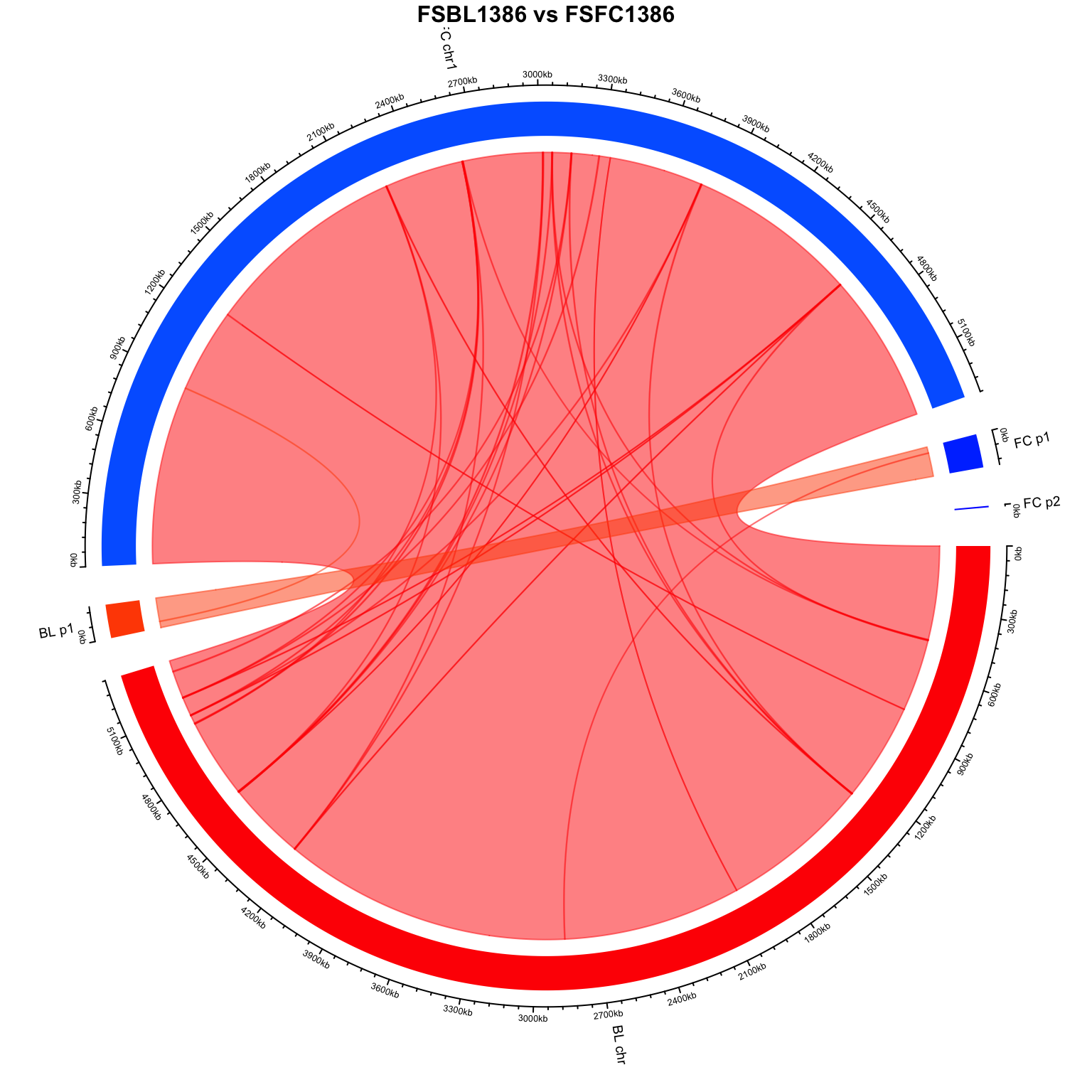
"#0066FF" "#0040FF" "#0019FF" "#FF0000" "#FF4D00"

2.7: Visualize with circlize

# Clear previous plots
circos.clear()
circos.par(gap.degree = 5)

# Initialize the genome data
circos.genomicInitialize(genome_lengths, plotType = "axis")

# Add a new track with different colors for each chromosome
circos.genomicTrackPlotRegion(genome_lengths, panel.fun = function(region, value, ...) {
  sector.index <- get.cell.meta.data("sector.index")
  col <- colors[sector.index]
  circos.genomicRect(region, value, col = col, border = NA)
}, bg.border = NA, track.height = 0.1, ylim = c(0, 1))

# Add custom sector labels with rotation
circos.track(track.index = 1, panel.fun = function(x, y) {
  sector.index <- get.cell.meta.data("sector.index")
  xcenter <- get.cell.meta.data("xcenter")
  circos.text(
    x = xcenter, 
    y = get.cell.meta.data("ylim")[1], 
    labels = sector.index, 
    facing = "reverse.clockwise", 
    niceFacing = TRUE, 
    adj = c(1.5, 0.5),
    cex = 0.6
  )
}, bg.border = NA)

# Plot the connections with specific colors
for (i in 1:nrow(blast_data)) {
  query_seq <- blast_data$qseqid[i]
  color <- colors[query_seq]
  
  circos.genomicLink(
    region1 = data.frame(chr = blast_data$qseqid[i], start = blast_data$qstart[i], end = blast_data$qend[i]),
    region2 = data.frame(chr = blast_data$sseqid[i], start = blast_data$sstart[i], end = blast_data$send[i]),
    col = adjustcolor(color, alpha.f = 0.5)
  )
}

# Add a title to the plot with increased text size
title(paste0(blood, " ", "vs", " ", faecal), cex.main = 1)