5: Analysing virulence factor determinants

Author

Richard Goodman

Published

April 24, 2025

Introduction

This tutorial screens genomes against the virulence factor database (VFDB) to search for virulence genes and visualises them as a heatmap.

It also shows how the BSI and DASSIM databases were compared.

Part 1 - Genome download and virulence factor screening with abricate

1.1: Download reads and run assemblies

See the code on how to download reads and run assemblies

1.2: Run abricate on genomes

Download abricate if you haven’t already, then you can run it simply with the following command.

abricate --db resfinder --mincov 60 --minid 90 --csv *.fasta > all_paired_blood_faecal_hybracter_vfdb_fasta_L60_T90_plus_BSI_indicators.csv

Part 2 - Plotting virulence factor heatmaps in R

2.1: Import the data

Import the data from abricate

library(readr)
library(dplyr)
library(tidyr)
library(pheatmap)
library(RColorBrewer)
library(readr)
library(reshape2)
library(pheatmap)
library(RColorBrewer)

# Reading in data
abricate_output = readr::read_csv("../data/all_paired_blood_faecal_hybracter_vfdb_fasta_L60_T90_plus_BSI_indicators.csv")

ab_tab = abricate_output

2.2: Wrangle abricate dataset

rm_duplicates = function(ab_tab)
{
  
  # First Remove duplicates
  # These cause issues with creating a lit rather than a dataframe
  # When compared against the database there can sometimes be duplciates 
  
  # arrange and group by ab_tab 
  ab_tab_unique <- ab_tab %>% 
    arrange(GENE, -`%COVERAGE`) %>% 
    group_by(GENE)
  
  # Check the colnames
  colnames(ab_tab_unique)
  
  # Check the duplicates 
  duplicated(ab_tab_unique[c("#FILE","GENE")])
  print("Duplicates found:")
  print(c(which(duplicated(ab_tab_unique[c("#FILE","GENE")]) == TRUE))) # see which contain duplicates
  
  # Remove columns that contain duplicates in FILE, GENE and COVERAGE 
  ab_tab_unique <- ab_tab[!duplicated(ab_tab_unique[c("#FILE","GENE")]),] #using colnames
  #ab_tab_unique <- ab_tab_unique[!duplicated(ab_tab_unique[c(1,2)]),] #using col numbers
  
  
  # Check whether duplicates have been delted 
  print("Duplicates remaining:")
  print(which(duplicated(ab_tab_unique[c("#FILE","GENE")]) == TRUE)) # see which contain duplicates
  
  {
    return(ab_tab_unique)
  }
}


# Run function 
ab_tab_unique = rm_duplicates(ab_tab)

[1] "Duplicates found:"
 [1] 404 405 406 407 408 409 410 411 412 413 414 415 416 417 418 419 420 421
[1] "Duplicates remaining:"
 [1] 724 728 729 733 734 736 740 741 745 748 749 751 752 754 757 758 760 764

mk_count_table = function(ab_tab)
{
  # Funtion to make the Abricate table wide 
  # Create a new value from original ab_tab to wide count table 
  wide = ab_tab %>% 
    # select strain, gene and resistance and rename
    select("#FILE", GENE, RESISTANCE) %>% 
    # rename 
    dplyr::rename(gene = "GENE",
           file = "#FILE",
           resistance = "RESISTANCE") %>% 
    # count genes vs strains
    count(file, gene) %>% 
    # Convert to wide table with genes as column headers and n as values 
    pivot_wider(names_from = gene,
                values_from = n)
  
  # Shorten strain names (remove the unnecessary string)
  wide$file = gsub(".fa", "", wide$file)
  wide$file = gsub("_assembled.fasta", "", wide$file)

  
  {
    return(wide)
  }
}

# Run function 
wide = mk_count_table(ab_tab_unique)

wide$file

 [1] "FSBL0558_hybractersta"  "FSBL1386_hybractersta"  "FSBL1448_flyesta"      
 [4] "FSBL1654_hybractersta"  "FSBL1925_hybractersta"  "FSBL2071_hybractersta" 
 [7] "FSBL2111_hybractersta"  "FSBL2112_hybractersta"  "FSBL2130_hybractersta" 
[10] "FSBL2155_hybractersta"  "FSBL2240_hybractersta"  "FSBL2258_hybractersta" 
[13] "FSBL2265_hybractersta"  "FSFC0558_hybractersta"  "FSFC1386_hybractersta" 
[16] "FSFC1448_flyesta"       "FSFC1654_unicyclersta"  "FSFC1925_hybractersta" 
[19] "FSFC2071_hybractersta"  "FSFC2111K_hybractersta" "FSFC2112_hybractersta" 
[22] "FSFC2130_hybractersta"  "FSFC2155_hybractersta"  "FSFC2240_unicyclersta" 
[25] "FSFC2258_hybractersta"  "FSFC2265_hybractersta"

wide$file <- gsub("_hybractersta", "", wide$file)
wide$file <- gsub("_flyesta", "", wide$file)
wide$file <- gsub("_unicyclersta", "", wide$file)

# check
wide$file

 [1] "FSBL0558"  "FSBL1386"  "FSBL1448"  "FSBL1654"  "FSBL1925"  "FSBL2071" 
 [7] "FSBL2111"  "FSBL2112"  "FSBL2130"  "FSBL2155"  "FSBL2240"  "FSBL2258" 
[13] "FSBL2265"  "FSFC0558"  "FSFC1386"  "FSFC1448"  "FSFC1654"  "FSFC1925" 
[19] "FSFC2071"  "FSFC2111K" "FSFC2112"  "FSFC2130"  "FSFC2155"  "FSFC2240" 
[25] "FSFC2258"  "FSFC2265"

# Converts to dataframe
count_to_dataframe = function(wide)
{
  wide = wide
  
  # make the genenames a variable 
  rows = wide$file
  
  # Remove the file column
  wide3 = wide %>% select(-file)
  
  # name the rows as strains
  rownames(wide3) = rows
  
  # convert to dataframe
  d = as.data.frame(wide3)
  
  # convert na to 0
  d[is.na(d)] = 0
  
  #name rows
  rownames(d) = rows
  
  # convert to matrix
  df = d
  
  
  {
    return(df)
  }
}

df = count_to_dataframe(wide)

# Converts to matrix
count_to_mat = function(wide)
{
  wide = wide
  
  # make the genenames a variable 
  rows = wide$file
  
  # Remove the file column
  wide3 = wide %>% select(-file)
  
  # name the rows as strains
  rownames(wide3) = rows
  
  # convert to dataframe
  d = as.data.frame(wide3)
  
  # convert na to 0
  d[is.na(d)] <- 0
  
  # name rows
  rownames(d) = rows
  
  # convert to matrix
  mat = as.matrix(d)
  
  
  {
    return(mat)
  }
}

# Run Function 
mat = count_to_mat(wide)


# Check output
nrow(mat)

[1] 26

class(mat)

[1] "matrix" "array"

colnames(mat)

 [1] "hha"       "yagZ/ecpA" "fyuA"      "irp1"      "irp2"      "ybtA"     
 [7] "ybtE"      "ybtP"      "ybtQ"      "ybtS"      "ybtT"      "ybtU"     
[13] "ybtX"      "aslA"      "chuA"      "chuS"      "chuT"      "chuU"     
[19] "chuV"      "chuW"      "chuX"      "chuY"      "entA"      "entB"     
[25] "entC"      "entD"      "entE"      "entF"      "entS"      "fdeC"     
[31] "fepA"      "fepB"      "fepC"      "fepD"      "fepG"      "fes"      
[37] "fimA"      "fimB"      "fimC"      "fimD"      "fimE"      "fimF"     
[43] "fimG"      "fimH"      "fimI"      "gspC"      "gspD"      "gspE"     
[49] "gspF"      "gspG"      "gspH"      "gspI"      "gspJ"      "gspK"     
[55] "gspL"      "gspM"      "iucA"      "iucB"      "iucC"      "iucD"     
[61] "kpsD"      "kpsM"      "kpsT"      "ompA"      "papB"      "papI"     
[67] "papX"      "sat"       "senB"      "vat"       "yagV/ecpE" "yagW/ecpD"
[73] "yagX/ecpC" "yagY/ecpB" "ykgK/ecpR" "afaB-I"    "afaC-I"    "daaF"     
[79] "draA"      "draD"      "draE2"     "draP"

rownames(mat)

 [1] "FSBL0558"  "FSBL1386"  "FSBL1448"  "FSBL1654"  "FSBL1925"  "FSBL2071" 
 [7] "FSBL2111"  "FSBL2112"  "FSBL2130"  "FSBL2155"  "FSBL2240"  "FSBL2258" 
[13] "FSBL2265"  "FSFC0558"  "FSFC1386"  "FSFC1448"  "FSFC1654"  "FSFC1925" 
[19] "FSFC2071"  "FSFC2111K" "FSFC2112"  "FSFC2130"  "FSFC2155"  "FSFC2240" 
[25] "FSFC2258"  "FSFC2265"

2.3: Plot a basic heatmap

Next we will select the mutations based

# convert to binary 
df = count_to_dataframe(wide)
df <- ifelse(df > 0, 1, 0)

# Generate  basic heatmap
pheatmap(df)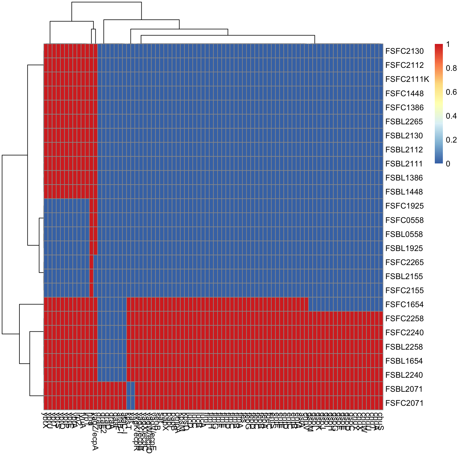

2.3: Plot an annotated heatmap

# Generate the heatmap with annotations

isolates = read_csv("../data/Isolate_species.csv")
  
isolates_df = as.data.frame(isolates)

isolates_df = isolates_df[-1,]

species_colors <- c("K. pneumoniae" = "#DDAD3B", 
                    "E. coli" = "#9F7831",
                    "K. quasipneumoniae similipneumoniae" = "#666666")

# Annotation for isolates (y-axis)
annotation_row <- data.frame(Species = isolates_df$Species)
rownames(annotation_row) <- isolates_df$Isolate

vfdb_class = read_csv("../data/VFDB_classes.csv")

vfdb_class_df = as.data.frame(vfdb_class)

class_colors <- c("Protectins" = "#4B9B7A", 
                  "Toxins" = "#CA6728", 
                  "Iron-uptake" = "#D43F88", 
                  "Adhesins" = "#7470AF")


# Annotation for isolates (x-axis)

annotation_col <- data.frame(class = vfdb_class_df$class)
rownames(annotation_col) <- vfdb_class_df$GENE

# Create a list of annotation colors
annotation_colors <- list(class = class_colors, Species = species_colors)


custom_colors <- colorRampPalette(c("#FFFFFF","#FBF5BB", "#FADF9F", "#F8B877", "#D37A5A", "#A84451"))(6)


pheatmap(df, 
         annotation_col = annotation_col, 
         annotation_row = annotation_row, 
         annotation_colors = annotation_colors, 
         color = custom_colors,
         show_rownames = TRUE, 
         show_colnames = TRUE,
         border_color = "black")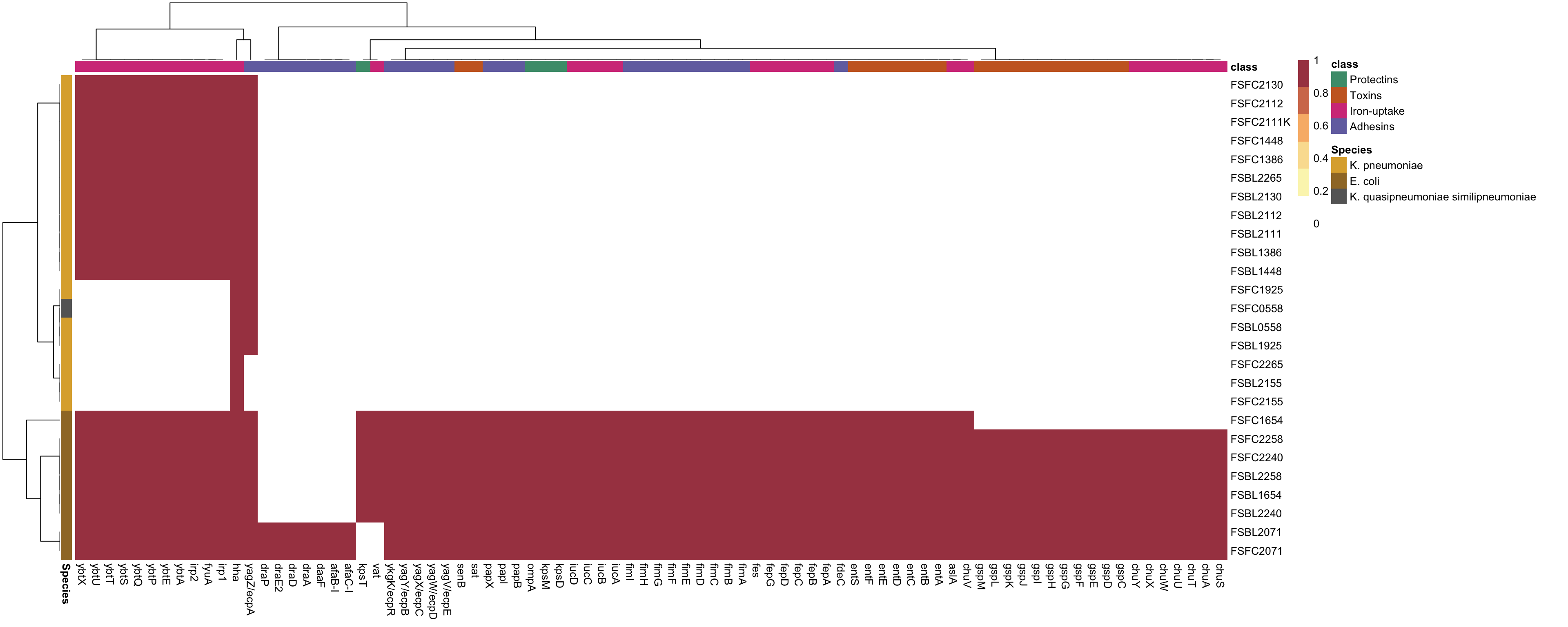

Part 3 - Comparison of virulence factors across datasets in R

3.1: Import the data

Import the data from abricate for 773 isolates from the BSI and DASSIM datasets.

# Load necessary libraries
library(readxl)
library(readr)
library(pheatmap)
library(dplyr)
library(tidyr)
library(tibble)
library(RColorBrewer)

# 772 Malawi Kleb Strains
abricate_output = readr::read_csv("../data/all_abricate_773_Ec_Kp_CHL_VFDB_fasta_L60_T90.csv")

ab_tab = abricate_output

#DASSIM <- DASSIM %>% select(matches("^ybt|^irp|^fyu"))

iron_VF <- ab_tab %>% filter(grepl("ybt|fyu|irp", GENE))

3.2: Wrangle dataset

# Remove duplicates 
ab_tab_unique = rm_duplicates(ab_tab)

[1] "Duplicates found:"
  [1]    67   630   750   754   757   761   770   788   793  3914  4276  4279
 [13]  4288  4291  4304  4319  4321  4482  4487  4497  4501  4515  4537  5093
 [25]  5130  5174  5221  5321  5880  5914  5915  5922  5975  6017  8089  8780
 [37]  9523  9759  9992 10037 10120 10123 10176 10195 10196 10197 10584 10598
 [49] 10600 10602 10603 10703 10711 10948 10949 12707 12949 13359 13503 13537
 [61] 13599 13667 14220 15243 15245 15320 15325 15389 15411 15456 15554 15606
 [73] 16078 17304 17306 17418 17425 17512 17593 17892 17919 18066 18068 18258
 [85] 18992 19318 20957 20958 21293 21648 22228 22317 22449 22560 22667 22673
 [97] 22674 23783 23785 23796 23798 23803 23822 23824 23855 23858 23882 23910
[109] 23912 23922 23935 23944 23995 24008 24012 24017 24020 24073 24075 24086
[121] 24088 24093 24112 24114 24145 24148 24172 24200 24202 24212 24225 24235
[133] 24300 25000 25095 25100 25103 25110 25376 26040 26104 26150 26213 26273
[145] 26325 26356 26359 26368 26371 26404 26407 26516 26518 26555 26559 26644
[157] 26647 26655 26666 26671 26673 26675 26677 26682 26686 26690 26692 26694
[169] 26701 26704 26706 26710 26720 26722 26726 26746 26749 26758 26762 26782
[181] 26866 26869 26899 26907 26909 26911 26913 26929 26933 26937 26948 26952
[193] 26974 27016 27267 27271 27272 28096 28133 28198 28364 28366 28876 28941
[205] 29050 29111 29641 29672 29673 29732 29797 30328 30365 30367 30375 30431
[217] 30538 31116 31151 31159 31213 31257 31283 34416 34417 34942 34977 34985
[229] 35040 35108 35171
[1] "Duplicates remaining:"
  [1]  1075  1083  1411  1414  3115  3116  3198  3199  3284  3967  3977  3978
 [13]  4220  4221  4406  4407  4885  4886  5738  6502  6504  7153  7154  7235
 [25]  7236  7692  7776  7779  7853  7859  7938  7941  8019  8022  8385  8422
 [37]  9591  9592  9593  9594  9597  9599  9609  9610  9998 10000 10002 10012
 [49] 10013 10014 10019 10508 10511 10624 10891 11065 11456 11457 11697 11698
 [61] 11945 11951 12493 12650 12948 12957 12958 14295 14328 14417 14418 14537
 [73] 14543 14999 15000 15143 15146 15152 15239 15240 15252 15253 15254 15291
 [85] 15298 15299 15300 15306 15307 15401 15430 15646 15647 15665 15685 15704
 [97] 15728 15792 15799 16387 16388 16389 16392 16393 16394 16398 17238 17239
[109] 18350 18351 18444 18445 18575 18606 18609 18930 19407 19413 19414 19627
[121] 19628 19934 19979 20757 20758 20759 20952 20953 21293 21720 21721 22104
[133] 22105 22672 22724 22725 23400 23427 23428 23431 23615 25109 25110 25118
[145] 25132 25566 25946 25964 25987 26450 26451 26494 26793 27176 27192 28250
[157] 28251 28274 28276 28277 28278 28279 28280 28801 28806 28818 28819 28820
[169] 28824 28883 28884 28891 28896 28901 28902 28903 28904 28905 28971 28977
[181] 28978 28979 28992 29884 29907 29908 29909 29917 29918 29919 29920 29921
[193] 29922 30323 30584 30594 30634 30635 30952 30971 30979 31031 32253 32262
[205] 32347 32358 32359 32485 32499 32500 32594 32652 32653 32787 32979 33063
[217] 33513 33514 33517 33533 33542 34034 34037 34038 34039 34040 34041 34089
[229] 34096

# Make count table
wide = mk_count_table(ab_tab_unique)

# Rename necessary 
wide$file = gsub("all_spades_assemblies/", "", wide$file)
wide$file = gsub(".fa", "", wide$file)
wide$file = gsub(".fasta", "", wide$file)
wide$file = gsub("_assembledsta", "", wide$file)
wide$file = gsub("_1_SPAdes_assemblysta", "", wide$file)
wide$file = gsub("_assembled.fasta", "", wide$file)
wide$file = gsub("_contigssta", "", wide$file)
wide$file = gsub("sta", "", wide$file)

# Convert count table to dataframe 
d = count_to_dataframe(wide)

# Convert count table to matrix
mat = count_to_mat(wide)

3.3: Filter for ybt + fyu + irp

# Filter the dataframe for the column "ybt"
#filtered_df <- d[, grepl("ybt", colnames(d)), drop = FALSE]
#filtered_df$seq = rownames(filtered_df)

# Filter the dataframe for columns containing "ybt", "fyu", or "irp"
filtered_df <- d[, grepl("ybt|fyu|irp", colnames(d)), drop = FALSE]

# Add row names as a new column
filtered_df$seq <- rownames(filtered_df)


# View the filtered dataframe
head(filtered_df)

            fyuA irp1 irp2 ybtA ybtE ybtP ybtQ ybtS ybtT ybtU ybtX         seq
26141-1-134    1    1    1    1    1    1    1    1    1    1    1 26141-1-134
26141-1-135    1    1    1    1    1    1    1    1    1    1    1 26141-1-135
26141-1-136    1    1    1    1    1    1    1    1    1    1    1 26141-1-136
26141-1-137    1    1    1    1    1    1    1    1    1    1    1 26141-1-137
26141-1-138    0    0    0    0    0    0    0    0    0    0    0 26141-1-138
26141-1-139    1    1    1    1    1    1    1    1    1    1    1 26141-1-139

# Sum values by category
library(dplyr)

3.4: Join to metadata

metadata = read_csv("../data/all_773_DASSIM_BSI_metadata.csv")
BSI_metadata_Ec = read_csv("../data/BSI_metadata_Ec.csv")
BSI_metadata_KpSc = read_csv("../data/BSI_metadata_KpSc_2.csv")

library(dplyr)
library(stringr)

filtered_df <- d[, grepl("ybt|fyu|irp", colnames(d)), drop = FALSE]
filtered_df$seq <- rownames(filtered_df)

filtered_df <- filtered_df %>%
  mutate(seq = gsub("-", "_", seq))

rownames(filtered_df) = gsub("-", "_", rownames(filtered_df))

# DASSIM    ERR3865256  28099_1_10  ERR3865256

# Create a named vector for replacement
replacement_map <- setNames(metadata$ENA_accession, metadata$lane)

# Perform the replacement
filtered_df <- filtered_df %>%
  mutate(accession = str_replace_all(seq, replacement_map) # Replace lanes with ENA accessions
  )

comparison_df = data.frame(accession = metadata$ENA_accession, 
                           lane = metadata$lane)

# Add the accession column with conditional logic
filtered_df[,"accession"] <- ifelse(
  grepl("^E", filtered_df[,"seq"]), # Check if seq starts with "E"
  filtered_df[,"seq"], # If true, copy seq to accession
  comparison_df$accession[match(unlist(filtered_df[,"seq"]), comparison_df$lane)] # Otherwise, match and replace
)

# View the results
print(filtered_df["28099_1_10",]) # Should be ERR3865256

           fyuA irp1 irp2 ybtA ybtE ybtP ybtQ ybtS ybtT ybtU ybtX        seq
28099_1_10    0    0    0    0    0    0    0    0    0    0    0 28099_1_10
            accession
28099_1_10 ERR3865256

# Reshape and summarize data for wide

metadata$accession = metadata$ENA_accession

metadata_Ec_update = metadata %>% 
  left_join(BSI_metadata_Ec, by = c('Strain_ID'))

metadata_KpSc_update = metadata_Ec_update %>% 
  left_join(BSI_metadata_KpSc, by = c('Strain_ID'))

meta_join = filtered_df %>% 
  left_join(metadata_KpSc_update, by = c('accession'))

# For KpSC

unique(meta_join$Species)

[1] "E. coli" NA        "KpSC"

meta_join_KpSc = meta_join %>% filter(Species == "KpSC")

unique(meta_join$study )

[1] "DASSIM"      NA            "bacteraemia"

DASSIM = meta_join_KpSc %>% filter(study == "DASSIM")
BSI = meta_join_KpSc %>% filter(study == "bacteraemia")

BSI = BSI %>% filter(Source.y == "Blood")

BSI$Source.y

 [1] "Blood" "Blood" "Blood" "Blood" "Blood" "Blood" "Blood" "Blood" "Blood"
[10] "Blood" "Blood" "Blood" "Blood" "Blood" "Blood" "Blood" "Blood" "Blood"
[19] "Blood" "Blood" "Blood" "Blood" "Blood" "Blood" "Blood" "Blood" "Blood"
[28] "Blood" "Blood" "Blood" "Blood" "Blood" "Blood" "Blood" "Blood" "Blood"
[37] "Blood" "Blood" "Blood" "Blood" "Blood" "Blood" "Blood" "Blood" "Blood"
[46] "Blood" "Blood" "Blood" "Blood" "Blood" "Blood" "Blood" "Blood" "Blood"
[55] "Blood" "Blood" "Blood"

#DASSIM = DASSIM %>% select(starts_with("ybt"))
#BSI= BSI %>% select(starts_with("ybt"))

DASSIM <- DASSIM %>% select(matches("^ybt|^irp|^fyu"))
BSI <- BSI %>% select(matches("^ybt|^irp|^fyu"))

summarized_DASSIM  <- DASSIM  %>% summarize(across(where(is.numeric), mean) * 100)
summarized_BSI <- BSI %>% summarize(across(where(is.numeric), mean) * 100)

summarized_DASSIM$study = "DASSIM"
summarized_BSI$study = "BSI"

# Reshape and summarize data
summarized_pc = rbind(summarized_DASSIM, summarized_BSI)

# Bar plot
library(ggplot2)
ggplot(summarized_pc, aes(x = study, y = ybtA, fill = study)) +
  geom_bar(stat = "identity") +
  labs(x = "Category", y = "Total Value", title = "Bar Plot by Protein Category") +
  theme_minimal()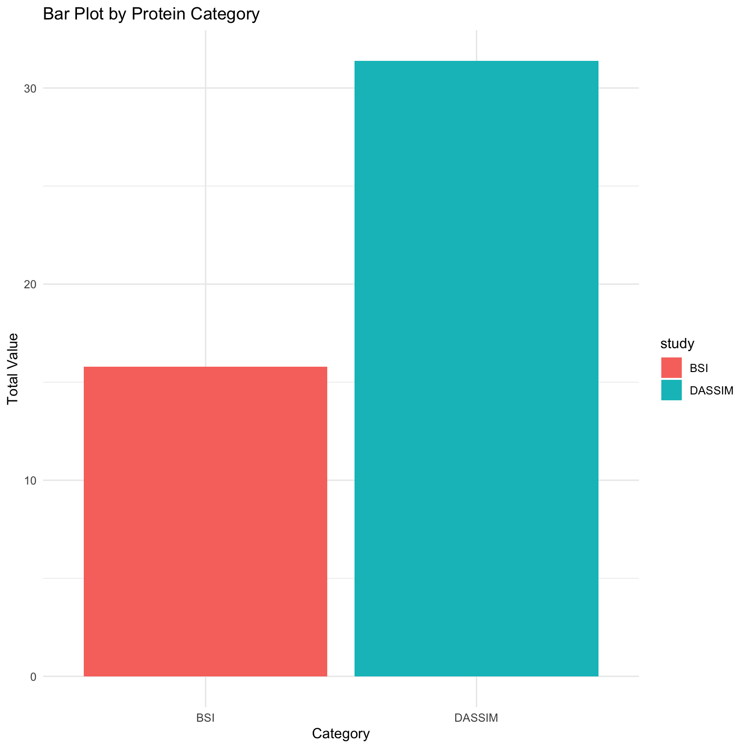

3.5: Join to DASSIM metadata

DASSIM_meta = read_csv("../data/DASSIM_metadata.csv")

library(dplyr)
library(stringr)


meta_join_DASSIM = meta_join %>% 
  left_join(DASSIM_meta, by = c('accession'))

3.6: Klebsiella pneumoniae species complex (KpSc)

# For KpSC

unique(meta_join_DASSIM$Species)

[1] "E. coli" NA        "KpSC"

meta_join_KpSc_DASSIM = meta_join_DASSIM %>% filter(Species == "KpSC")

unique(meta_join$study)

[1] "DASSIM"      NA            "bacteraemia"

DASSIM = meta_join_KpSc_DASSIM %>% filter(study == "DASSIM")
DASSIM_sepsis = DASSIM %>% filter(condition == "sepsis")
DASSIM_inpatient = DASSIM %>% filter(condition == "inpatient")
DASSIM_community = DASSIM %>% filter(condition == "community")
BSI = meta_join_KpSc_DASSIM %>% filter(study == "bacteraemia")
BSI = BSI %>% filter(Source.y == "Blood")

#DASSIM_sepsis = DASSIM_sepsis %>% select(starts_with("ybt"))
#DASSIM_inpatient = DASSIM_inpatient %>% select(starts_with("ybt"))
#DASSIM_community = DASSIM_community %>% select(starts_with("ybt"))
#BSI = BSI %>% select(starts_with("ybt"))


# Select columns that start with "ybt", "adr", or "ppy"
DASSIM_sepsis = DASSIM_sepsis %>% select(matches("^ybt|^irp|^fyu"))
DASSIM_inpatient = DASSIM_inpatient %>% select(matches("^ybt|^irp|^fyu"))
DASSIM_community = DASSIM_community %>% select(matches("^ybt|^irp|^fyu"))
BSI = BSI %>% select(matches("^ybt|^irp|^fyu"))


nrow(DASSIM_sepsis) # 138

[1] 138

nrow(DASSIM_inpatient) # 33

[1] 33

nrow(DASSIM_community) # 16

[1] 16

nrow(BSI) # 57

[1] 57

# summarized_DASSIM_sepsis = DASSIM_sepsis %>% summarize(across(where(is.numeric), mean) * 100)

summarized_DASSIM_sepsis = DASSIM_sepsis %>% summarize(across(where(is.numeric), ~ sum(. == 1) / n() * 100))
summarized_DASSIM_inpatient = DASSIM_inpatient %>% summarize(across(where(is.numeric), ~ sum(. == 1) / n() * 100))
summarized_DASSIM_community = DASSIM_community %>% summarize(across(where(is.numeric), ~ sum(. == 1) / n() * 100))
summarized_BSI <- BSI %>% summarize(across(where(is.numeric), ~ sum(. == 1) / n() * 100))


summarized_DASSIM_sepsis$study = "DASSIM_sepsis"
summarized_DASSIM_inpatient$study = "DASSIM_inpatient"
summarized_DASSIM_community$study = "DASSIM_community"
summarized_BSI$study = "BSI"

# Reshape and summarize data
summarized_pc = rbind(summarized_DASSIM_sepsis, summarized_DASSIM_inpatient, summarized_DASSIM_community, summarized_BSI)

# Bar plot
library(ggplot2)
ggplot(summarized_pc, aes(x = study, y = ybtA, fill = study)) +
  geom_bar(stat = "identity") +
  labs(x = "Category", y = "Total Value", title = "Bar Plot by Protein Category") +
  theme_minimal()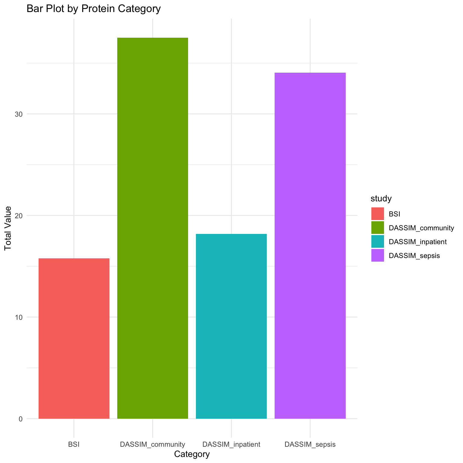

# Convert to long  ##

summarized_long_pc = summarized_pc %>% pivot_longer(!study, names_to = "gene", values_to = "count")

summarized_pc_for_paper_KpSc = summarized_long_pc %>% group_by(study) %>% summarize(meant_count = mean(count))

summarized_long_pc$order <- factor(summarized_long_pc$study, levels = sort(unique(summarized_long_pc$study)))

level_order <- c('BSI', 'DASSIM_inpatient', 'DASSIM_sepsis', "DASSIM_community") 

KPSC_plot = ggplot(summarized_long_pc, aes(x = factor(study, level = level_order), y = count, fill = study)) +
  geom_bar(stat = "identity") +
  ylim(0, 100) +
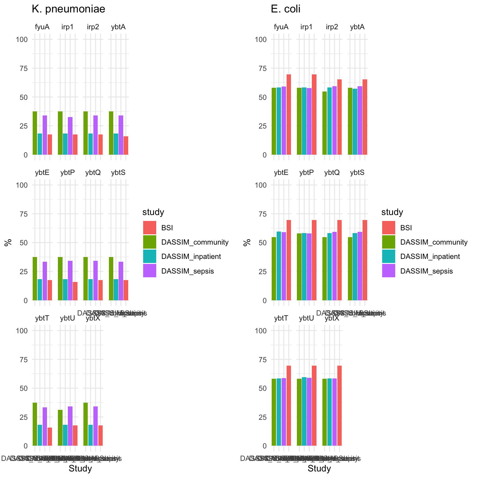
  labs(x = "Study", y = "%", title = "K. pneumoniae") +
  theme_minimal() + facet_wrap(~ gene)
KPSC_plot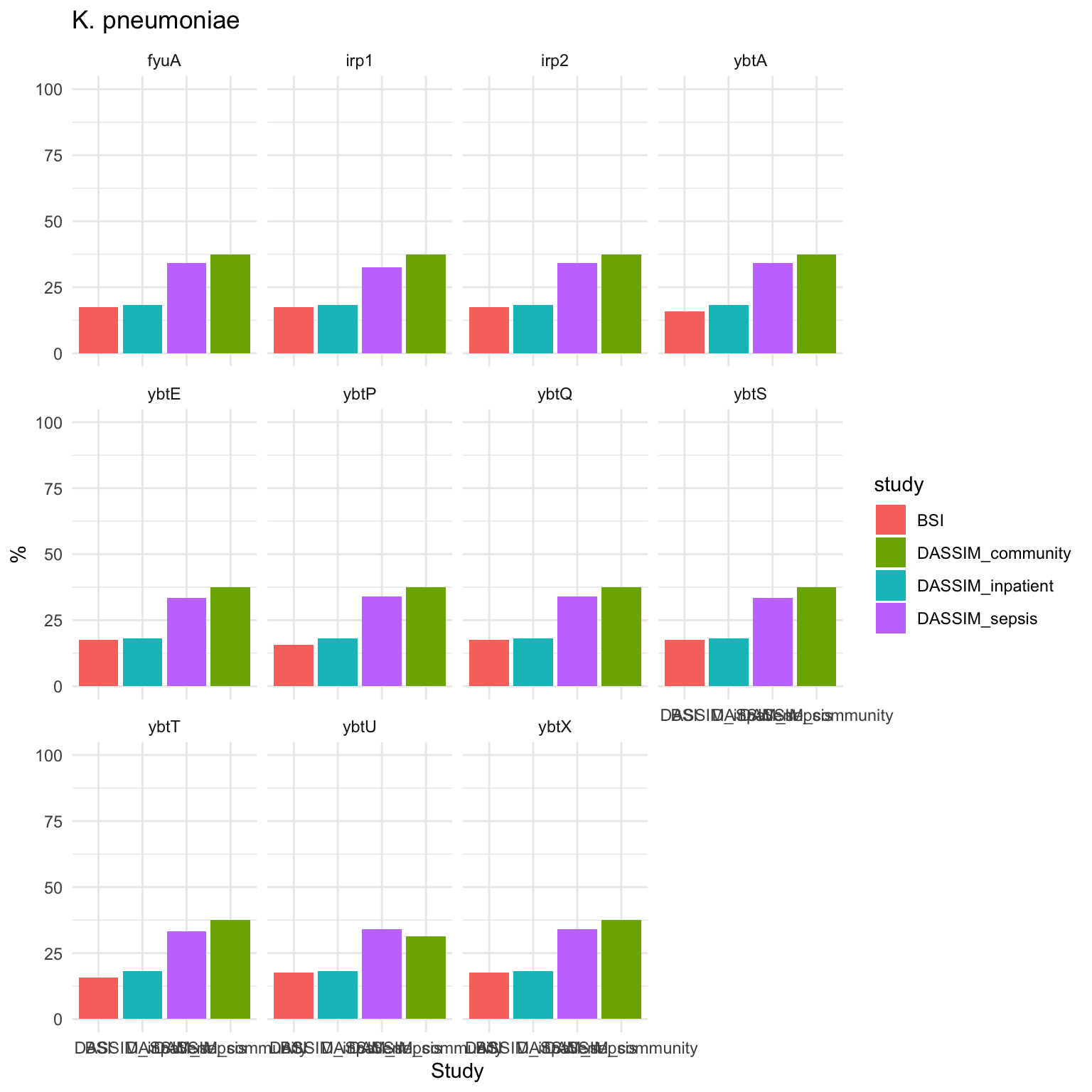

3.7: E. coli

# For Ecoli

unique(meta_join_DASSIM$Species)

[1] "E. coli" NA        "KpSC"

meta_join_Ecoli_DASSIM = meta_join_DASSIM %>% filter(Species == "E. coli")

unique(meta_join$study)

[1] "DASSIM"      NA            "bacteraemia"

DASSIM = meta_join_Ecoli_DASSIM %>% filter(study == "DASSIM")
DASSIM_sepsis = DASSIM %>% filter(condition == "sepsis")
DASSIM_inpatient = DASSIM %>% filter(condition == "inpatient")
DASSIM_community = DASSIM %>% filter(condition == "community")
BSI = meta_join_Ecoli_DASSIM %>% filter(study == "bacteraemia")
BSI = BSI %>% filter(Source.x == "Blood")

#DASSIM_sepsis = DASSIM_sepsis %>% select(starts_with("ybt"))
#DASSIM_inpatient = DASSIM_inpatient %>% select(starts_with("ybt"))
#DASSIM_community = DASSIM_community %>% select(starts_with("ybt"))
#BSI = BSI %>% select(starts_with("ybt"))


DASSIM_sepsis = DASSIM_sepsis %>% select(matches("^ybt|^irp|^fyu"))
DASSIM_inpatient = DASSIM_inpatient %>% select(matches("^ybt|^irp|^fyu"))
DASSIM_community = DASSIM_community %>% select(matches("^ybt|^irp|^fyu"))
BSI = BSI %>% select(matches("^ybt|^irp|^fyu"))

nrow(DASSIM_sepsis) # 334

[1] 334

nrow(DASSIM_inpatient) # 84

[1] 84

nrow(DASSIM_community) # 31

[1] 31

nrow(BSI) # 23

[1] 23

# summarized_DASSIM_sepsis = DASSIM_sepsis %>% summarize(across(where(is.numeric), mean) * 100)

summarized_DASSIM_sepsis = DASSIM_sepsis %>% summarize(across(where(is.numeric), ~ sum(. == 1) / n() * 100))
summarized_DASSIM_inpatient = DASSIM_inpatient %>% summarize(across(where(is.numeric), ~ sum(. == 1) / n() * 100))
summarized_DASSIM_community = DASSIM_community %>% summarize(across(where(is.numeric), ~ sum(. == 1) / n() * 100))
summarized_BSI <- BSI %>% summarize(across(where(is.numeric), ~ sum(. == 1) / n() * 100))

summarized_DASSIM_sepsis$study = "DASSIM_sepsis"
summarized_DASSIM_inpatient$study = "DASSIM_inpatient"
summarized_DASSIM_community$study = "DASSIM_community"
summarized_BSI$study = "BSI"

# Reshape and summarize data
summarized_pc = rbind(summarized_DASSIM_sepsis, summarized_DASSIM_inpatient, summarized_DASSIM_community, summarized_BSI)

# Bar plot
library(ggplot2)
ggplot(summarized_pc, aes(x = study, y = ybtA, fill = study)) +
  geom_bar(stat = "identity") +
  labs(x = "Category", y = "Total Value", title = "Bar Plot by Protein Category") +
  theme_minimal()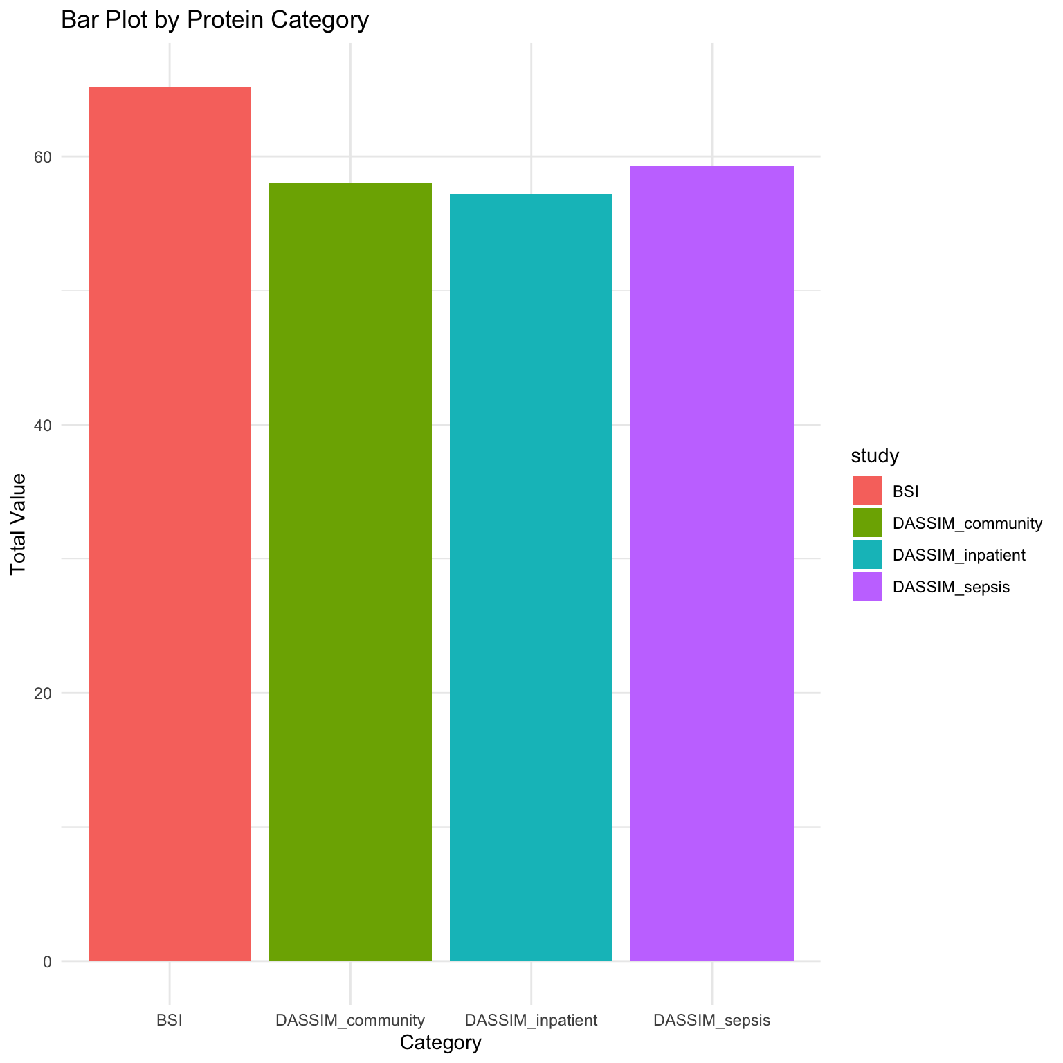

# Convert to long  ##

summarized_long_pc = summarized_pc %>% pivot_longer(!study, names_to = "gene", values_to = "count")

summarized_pc_for_paper_Ec = summarized_long_pc %>% group_by(study) %>% summarize(meant_count = mean(count))

summarized_long_pc$order <- factor(summarized_long_pc$study, levels = sort(unique(summarized_long_pc$study)))

level_order <- c("DASSIM_community", 'DASSIM_inpatient', 'DASSIM_sepsis', 'BSI') 

Ecoli_plot = ggplot(summarized_long_pc, aes(x = factor(study, level = level_order), y = count, fill = study)) +
  geom_bar(stat = "identity") +
  ylim(0, 100) +
  labs(x = "Study", y = "%", title = "E. coli") +
  theme_minimal() + facet_wrap(~ gene)
Ecoli_plot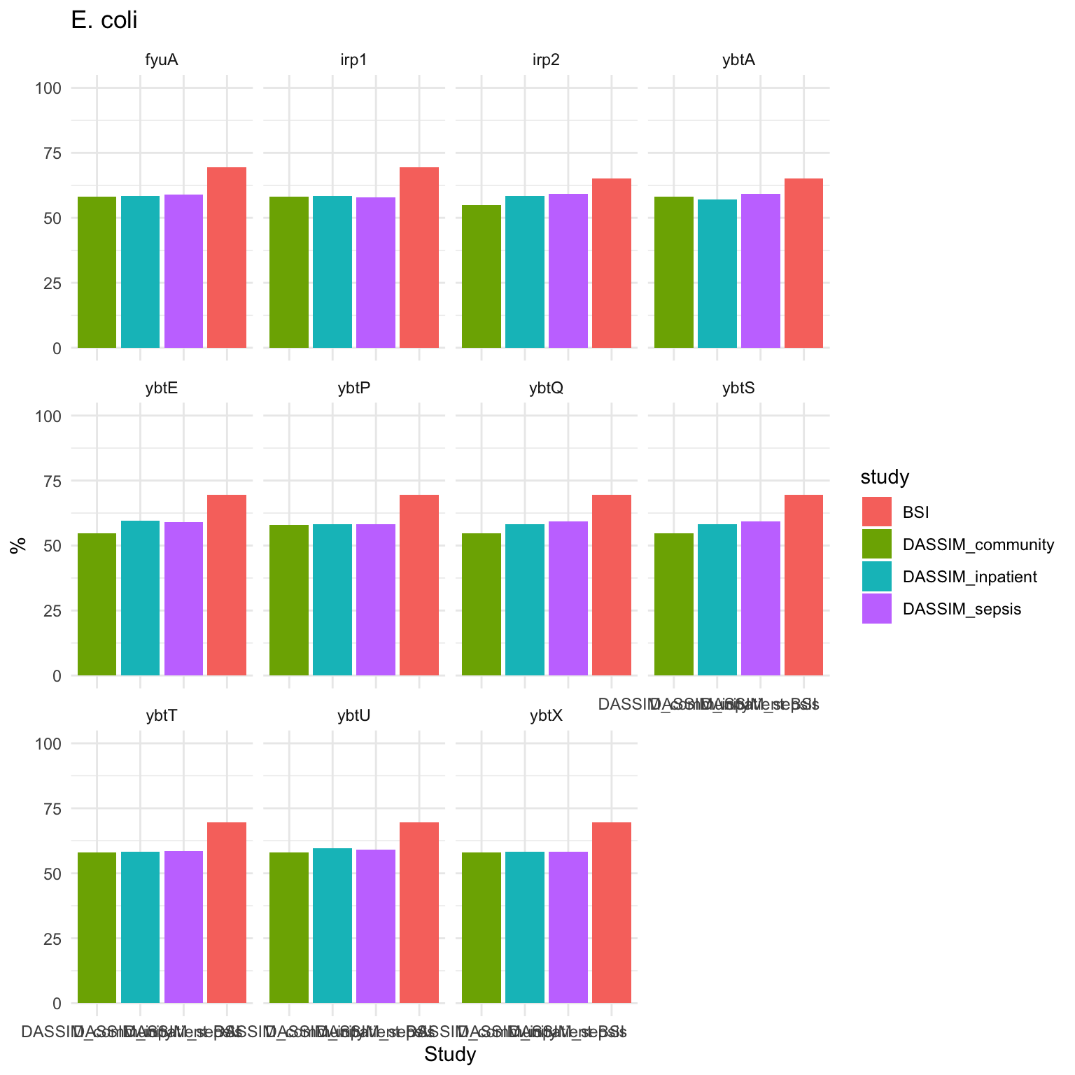

3.8: E. coli and KpSc plotted together

library(ggpubr)
ggarrange(KPSC_plot, Ecoli_plot, ncol = 2, nrow = 1)