Geospatial mapping of waterways in Jakarta, Indonesia

Author

Richard Goodman

Published

July 4, 2025

1. Setting up R

library(sf)
library(ggplot2)
library(osmdata)
library(readxl)
library(dplyr)
library(rnaturalearth)
library(rnaturalearthdata)
library(viridis)
library(tidyr)   # For pivoting
library(ggforce) # For pie charts
library(ggrepel)
library(stringr)
library(scatterpie)

2. Loading data

# 1. Read data
metadata = read.csv("../data/metadata_all_edit2.csv")
locations = read_excel("../data/GPS Data of Environment sampling site_TC.xlsx")

3. Wrangle data

# Remove number before locations
locations =  locations %>%
  mutate(site = sub("^[0-9]+\\.", "", Location))

locations[locations$Location == "Pasar Sawah Barat", "Longitude"] = 106.93

# create a new column with mutations 
metadata =  metadata %>%
  dplyr::mutate(site = sub("^[0-9]+\\.", "", site))

# Merge metadata and coordinates
metadata_mlst = metadata %>%
  dplyr::left_join(locations, by = c("site" = "site"))

# Choose 
metadata_mlst_2 = metadata_mlst %>%
  dplyr::filter(sector == "Human" | sector == "Environment" | sector == "Animal")

4. Making the Jakarta Map

# boundaries
gj_bbox = c(xmin = 106.5, ymin = -6.7, xmax = 107.2, ymax = -5.9)

# Query for city/regency boundaries (admin level 5)
greater_jakarta_admin = opq(bbox = gj_bbox) %>%
  add_osm_feature(key = "admin_level", value = "5") %>%
  osmdata_sf()

greater_jakarta_map = greater_jakarta_admin$osm_multipolygons

#plot(st_geometry(greater_jakarta_map))

unique(greater_jakarta_map$name)

 [1] "Jakarta Selatan"     "Jakarta Timur"       "Kepulauan Seribu"   
 [4] "Jakarta Pusat"       "Jakarta Barat"       "Jakarta Utara"      
 [7] "Tangerang Selatan"   "Tangerang"           "Kabupaten Tangerang"
[10] "Bekasi"              "Depok"               "Bogor"              
[13] "Kab Bogor"           "Kab Bekasi"          "Cianjur"            
[16] "Karawang"

unique(greater_jakarta_map$admin_level)

[1] "5"

unique(greater_jakarta_map$type)

[1] "boundary"

gj_filtered = greater_jakarta_map %>%
  filter(grepl("Jakarta|Bogor|Bekasi|Depok|Tangerang", name))

labels_df = gj_filtered %>%
  st_point_on_surface() %>%  # safer than centroid for oddly shaped areas
  select(name) %>%
  mutate(lon = st_coordinates(.)[,1],
         lat = st_coordinates(.)[,2])

Warning: st_point_on_surface assumes attributes are constant over geometries

Warning in st_point_on_surface.sfc(st_geometry(x)): st_point_on_surface may not
give correct results for longitude/latitude data

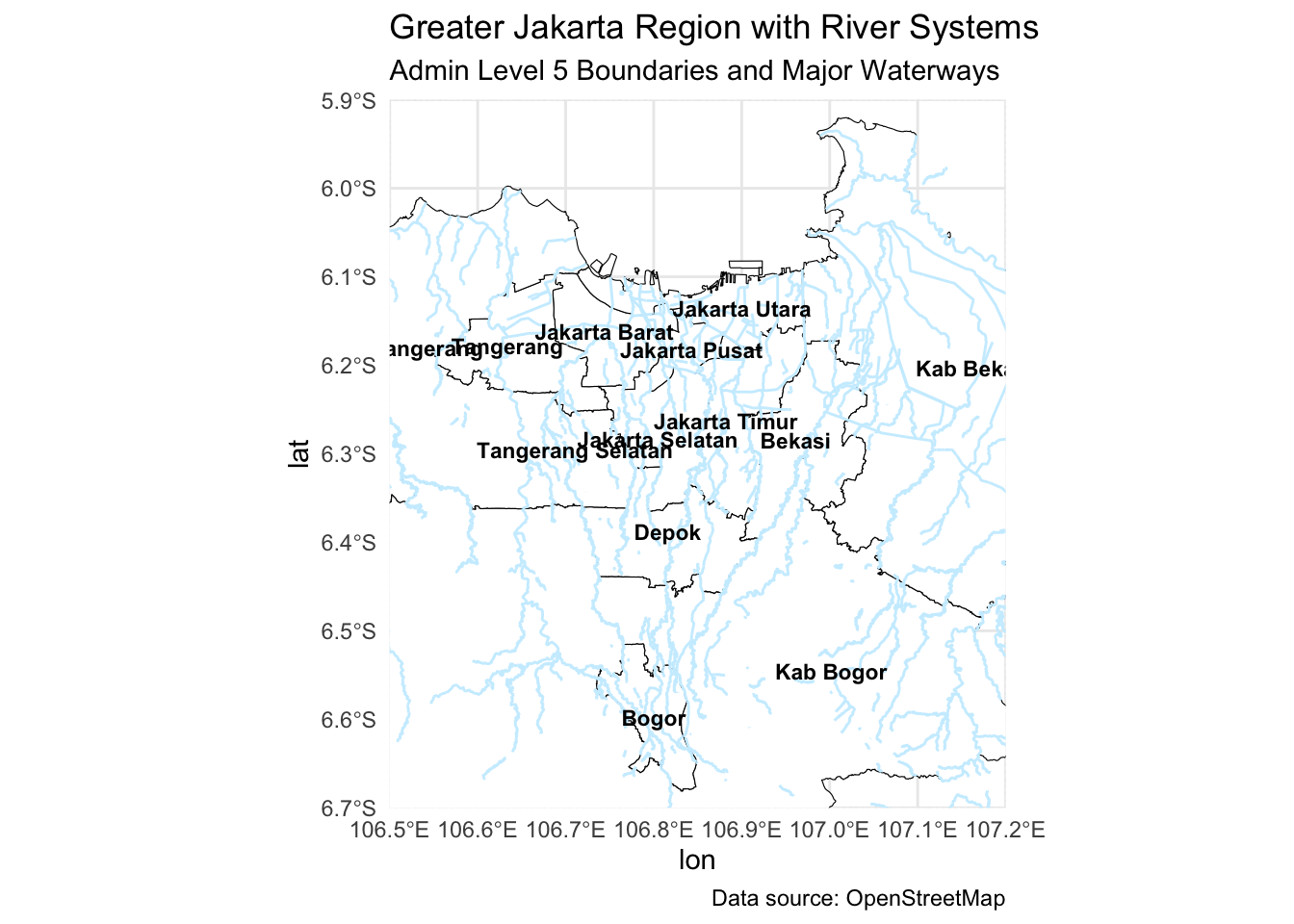
5. Making the Jakarta Map with rivers

coords = read.csv("../data/metadata_combined_with_mlst_human_animal_env.csv")

# Step 1: Query OSM for river systems within the Jakarta bounding box
gj_waterways = opq(bbox = gj_bbox) %>%
  add_osm_feature(key = "waterway") %>%
  osmdata_sf()

# Step 2: Extract the 'lines' layer (rivers, canals, streams are linear features)
gj_rivers = gj_waterways$osm_lines

# Optional: Filter for specific types of waterways (optional but can help declutter)
gj_rivers = gj_rivers %>%
  filter(waterway %in% c("river", "canal", "stream"))

gj_rivers = gj_rivers %>%
  filter(waterway %in% c("river"))

river_labels = gj_rivers %>%
  filter(!is.na(name)) %>%                # Keep only named rivers
  group_by(name) %>%
  dplyr::slice(1) %>%                            # Only one label per river
  ungroup() %>%
  st_point_on_surface() %>%
  mutate(lon = st_coordinates(.)[, 1],
         lat = st_coordinates(.)[, 2])

Warning: st_point_on_surface assumes attributes are constant over geometries

Warning in st_point_on_surface.sfc(st_geometry(x)): st_point_on_surface may not
give correct results for longitude/latitude data

sunter_river = gj_rivers %>%
  filter(name %in% c("Sunter River", "Sunter", "Kali Sunter"))


ciliwung_river = gj_rivers %>%
  filter(name %in% c("Ciliwung River", "Ciliwung", "Kali Ciliwung"))


cipinang_river = gj_rivers %>%
  filter(name %in% c("Cipinang River", "Cipinang", "Kali Cipinang"))


BKT = gj_rivers %>%
  filter(name %in% c("BKT", "Banjir Kanal Timur", "Kanal Banjir Barat", "Kanal Banjir Timur"))



cakung_drain = gj_rivers %>%
  filter(name %in% c("Cakung"))



# Step 3: Plot with rivers overlaid
ggplot() +
  geom_sf(data = gj_filtered, fill = "white", color = "black") +  # city/regency areas
  geom_sf(data = gj_rivers, color = "#cceeff", size = 1) +              # rivers
  geom_text(data = labels_df, aes(x = lon, y = lat, label = name), size = 3, fontface = "bold")  +
  coord_sf(xlim = c(106.5, 107.2), ylim = c(-6.7, -5.9), expand = FALSE) +
  labs(title = "Greater Jakarta Region with River Systems",
       subtitle = "Admin Level 5 Boundaries and Major Waterways",
       caption = "Data source: OpenStreetMap") +
  theme_minimal()

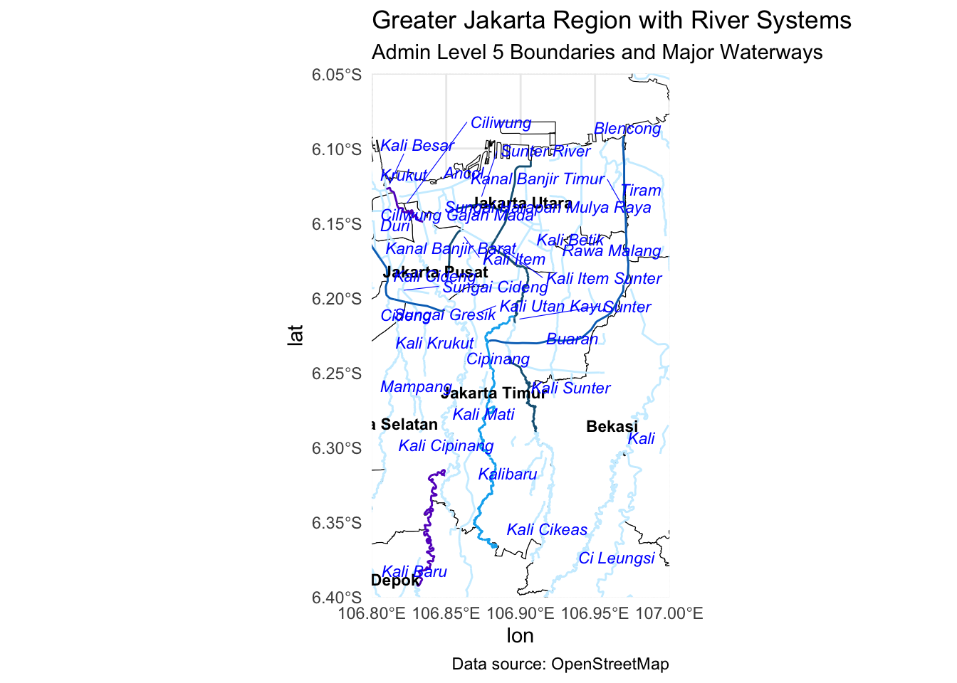
ggplot() +
  geom_sf(data = gj_filtered, fill = "white", color = "black") +  # city/regency areas
  geom_sf(data = gj_rivers, color = "#cceeff", size = 5) +
  geom_sf(data = sunter_river, color = "#176082", size = 5) + 
  geom_sf(data = ciliwung_river, color = "#6713C6", size = 5) +
  geom_sf(data = cipinang_river, color = "#00B0F0", size = 5) +  
  geom_sf(data = BKT, color = "#0070C0", size = 5) + # rivers
  geom_text(data = labels_df, aes(x = lon, y = lat, label = name), size = 3, fontface = "bold")  +
  geom_text_repel(
    data = river_labels,
    aes(x = lon, y = lat, label = name),
    size = 3, fontface = "italic", color = "blue",
    segment.color = "blue", segment.size = 0.2,
    box.padding = 0.3, point.padding = 0.3, max.overlaps = Inf
  ) +
  coord_sf(xlim = c(106.8, 107.0), ylim = c(-6.4, -6.05), expand = FALSE) +
  labs(title = "Greater Jakarta Region with River Systems",
       subtitle = "Admin Level 5 Boundaries and Major Waterways",
       caption = "Data source: OpenStreetMap") +
  theme_minimal()

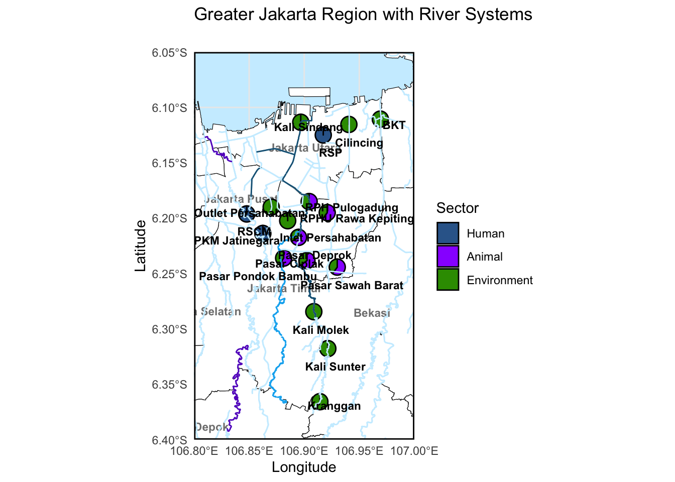
# Step 3: Plot with rivers overlaid and sample sites
pie_df= coords %>%
  dplyr::count(Longitude, Latitude, sector) %>%   # Count samples per sector per location
  pivot_wider(
    names_from = sector,
    values_from = n,
    values_fill = 0  )                      # Fill missing sector values with 0

pie_labels = coords %>%
  distinct(site, Longitude, Latitude) %>%
  mutate(
    label_lon = Longitude + 0.01,   # Offset east
    label_lat = Latitude - 0.01     # Offset north
  )


sector_key = unique(coords[, c("sector", "sector_colour")])


p_rivers = ggplot() +
  geom_sf(data = gj_filtered, fill = "white", color = "black") +  # city/regency areas
  geom_sf(data = gj_rivers, color = "#cceeff", size = 5) +              # rivers
  geom_text(data = labels_df,
            aes(x = lon, y = lat, label = name),
            size = 3, fontface = "bold", color = "gray50") +
  geom_scatterpie(
    data = pie_df,
    aes(x = Longitude, y = Latitude),
    cols = sector_key$sector,    # a character vector of your sector names
    pie_scale = 3) +                   # adjust this so pies aren’t too big/small   
  geom_sf(data = gj_rivers, color = "#cceeff", size = 5) +
  geom_sf(data = sunter_river, color = "#176082", size = 5) + 
  geom_sf(data = ciliwung_river, color = "#6713C6", size = 5) +
  geom_sf(data = cipinang_river, color = "#00B0F0", size = 5) +
  scale_fill_manual(
    name   = "Sector",
    values = setNames(sector_key$sector_colour,
                      sector_key$sector)) +
  geom_text_repel(data = pie_labels,
                  aes(x = label_lon, y = label_lat, label = site),
                  size = 3, fontface = "bold", color = "black",
                  box.padding = 0, point.padding = 0, max.overlaps = Inf,
                  segment.color = "gray50", segment.size = 1, force = 4) +
  coord_sf(
    xlim = c(106.8, 107.0),
    ylim = c(-6.4, -6.05), expand = FALSE) +
  theme_minimal()  + 
  theme(
    panel.background = element_rect(fill = "#cceeff", color = NA)) +
  theme(legend.position = "right",
        panel.border = element_rect(colour = "black", fill=NA, linewidth=1)) +
  labs(title = "Greater Jakarta Region with River Systems",
       subtitle = " ",
       x = "Longitude", y = "Latitude")


# 5. Print the map
print(p_rivers)

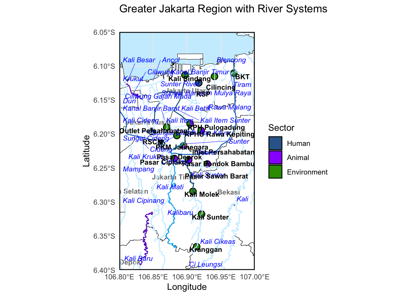
ggsave("../imgs/Greater Jakarta Region with River Systems and sample sites.svg", p_rivers, height = 8, width = 8)
ggsave("../imgs/Greater Jakarta Region with River Systems and sample sites.png", p_rivers, height = 8, width = 8)



p_rivers_highlights = ggplot() +
  geom_sf(data = gj_filtered, fill = "white", color = "black") +  # city/regency areas
  geom_sf(data = gj_rivers, color = "#cceeff", size = 5) +              # rivers
  geom_text(data = labels_df,
            aes(x = lon, y = lat, label = name),
            size = 3, fontface = "bold", color = "gray50") +
  geom_scatterpie(
    data = pie_df,
    aes(x = Longitude, y = Latitude),
    cols = sector_key$sector,    # a character vector of your sector names
    pie_scale = 2) +                   # adjust this so pies aren’t too big/small   
  geom_sf(data = gj_rivers, color = "#cceeff", size = 5) +
  geom_sf(data = sunter_river, color = "#176082", size = 5) + 
  geom_sf(data = ciliwung_river, color = "#6713C6", size = 5) + 
  geom_sf(data = cipinang_river, color = "#00B0F0", size = 5) +  
  geom_sf(data = BKT, color = "#0070C0", size = 5) + 
  scale_fill_manual(
    name   = "Sector",
    values = setNames(sector_key$sector_colour,
                      sector_key$sector)) + 
  geom_text_repel(
    data = river_labels,
    aes(x = lon, y = lat, label = name),
    size = 3, fontface = "italic", color = "blue",
    segment.color = "blue", segment.size = 0.2,
    box.padding = 0.3, point.padding = 0.3, max.overlaps = Inf
  ) +
  geom_text_repel(data = pie_labels,
                  aes(x = label_lon, y = label_lat, label = site),
                  size = 3, fontface = "bold", color = "black",
                  box.padding = 0, point.padding = 0, max.overlaps = Inf,
                  segment.color = "gray50", segment.size = 1, force = 4) +
  coord_sf(
    xlim = c(106.8, 107.0),
    ylim = c(-6.4, -6.05), expand = FALSE) +
  theme_minimal()  + 
  theme(
    panel.background = element_rect(fill = "#cceeff", color = NA)) +
  theme(legend.position = "right",
        panel.border = element_rect(colour = "black", fill=NA, linewidth=1)) +
  labs(title = "Greater Jakarta Region with River Systems",
       subtitle = " ",
       x = "Longitude", y = "Latitude")


print(p_rivers_highlights)

ggsave("../imgs/Greater Jakarta Region with River Systems and sample sites main rivers highlighted.svg", p_rivers_highlights, height = 8, width = 8)
ggsave("../imgs/Greater Jakarta Region with River Systems and sample sites main rivers highlighted.png", p_rivers_highlights, height = 8, width = 8)